Reading in data and basic data manipulation using R

Getting started

In this page we will get started using R to read in data, installing packages, and manipulating data.

To read in our data, we will use R’s tidyverse family of libraries. Before we begin, let’s make sure that we have the most recent version of tidyverse installed:

install.packages(“tidyverse”)

Depending on when you last updated your computer this may, or may not, result in a bunch of output about installing the package.

Next, let’s load the library:

library(tidyverse)

── Attaching core tidyverse packages ──────────────────────── tidyverse 2.0.0 ──
✔ dplyr     1.1.4     ✔ readr     2.1.5
✔ forcats   1.0.0     ✔ stringr   1.5.1
✔ ggplot2   3.5.1     ✔ tibble    3.2.1
✔ lubridate 1.9.3     ✔ tidyr     1.3.1
✔ purrr     1.0.2     
── Conflicts ────────────────────────────────────────── tidyverse_conflicts() ──
✖ dplyr::filter() masks stats::filter()
✖ dplyr::lag()    masks stats::lag()
ℹ Use the conflicted package (<http://conflicted.r-lib.org/>) to force all conflicts to become errors

The output that follows library("tidyverse") is fairly typical and is R’s way of telling you that if you type in certain commands, such as filter, you may get the results of a different function than the one that you expected. The double colon notation (::) is a way to make sure that you got the version of the command that you wanted to use. So if you wanted to use the filter command from the stats package after this you would type stats::filter instead of just filter.

Reading data with R

Now that we have loaded the tidyverse, let’s go get the data file. For this example, we are using a cleaned dataset that I have created from the National Health Interview Survey to demonstrate how insurance coverage changes over time. This file is located at https://andersen-hecon.github.io/data/nhis_for_example.csv and we can load the file (and assign it to the name data) using the code:

data<-read_csv(“https://andersen-hecon.github.io/data/nhis_for_example.csv”)

As you can see below, executing this code results in R providing some data about the file–in particular the “Delimiter,” or how the columns of data are divided (commas in this case), and the types and names of the columns.

Rows: 4128 Columns: 9
── Column specification ────────────────────────────────────────────────────────
Delimiter: ","
chr (1): sex
dbl (8): year, age, pop, any_insurance, private_insurance, chip_insurance, m...

ℹ Use `spec()` to retrieve the full column specification for this data.
ℹ Specify the column types or set `show_col_types = FALSE` to quiet this message.

We can suppress (or eliminate) this information using the option “show_col_types=FALSE” so that the code would read:

data<-read_csv(“https://andersen-hecon.github.io/data/nhis_for_example.csv”, show_col_types=FALSE)

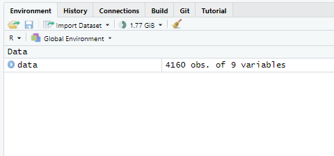
Notice now that we have loaded the file that it appears in the environment window in the top right corner of the RStudio window:

Summarizing data

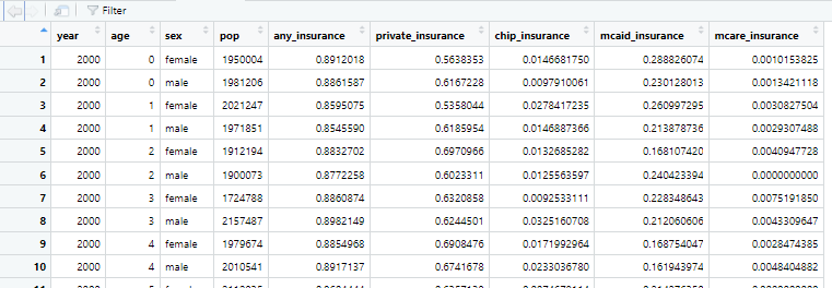
We can look at the data we have loaded in several ways. The easiest (in RStudio) is to use the viewer either by clicking on the data object in the environment window or by typing View(data) in the console window. These ways of viewing the data provide a detailed, line by line, view of the data. We can achieve something similar by typing data or print(data) at the console:

# A tibble: 4,128 × 9
    year   age sex        pop any_insurance private_insurance chip_insurance
   <dbl> <dbl> <chr>    <dbl>         <dbl>             <dbl>          <dbl>
 1  2000     0 female 1950004         0.891             0.564        0.0147 
 2  2000     0 male   1981206         0.886             0.617        0.00979
 3  2000     1 female 2021247         0.860             0.536        0.0278 
 4  2000     1 male   1971851         0.855             0.619        0.0147 
 5  2000     2 female 1912194         0.883             0.697        0.0133 
 6  2000     2 male   1900073         0.877             0.602        0.0126 
 7  2000     3 female 1724788         0.886             0.632        0.00925
 8  2000     3 male   2157487         0.898             0.624        0.0325 
 9  2000     4 female 1979674         0.885             0.691        0.0172 
10  2000     4 male   2010541         0.892             0.674        0.0233 
# ℹ 4,118 more rows
# ℹ 2 more variables: mcaid_insurance <dbl>, mcare_insurance <dbl>

Please pay careful attention to the last line of the output (“# ℹ 2 more variables: mcaid_insurance , mcare_insurance ”), which indicate that the screen wasn’t wide enough to show two of the variables (mcaid_insurace and mcare_insurance). Viewing the data allows us to see more variables and columns in RStudio:

Lastly, we can use the summary command to get some characteristics about the data and each variable by typing summary(data) at the console:

      year           age           sex                 pop         
 Min.   :2000   Min.   : 0.0   Length:4128        Min.   : 192055  
 1st Qu.:2006   1st Qu.:21.0   Class :character   1st Qu.:1609411  
 Median :2012   Median :42.5   Mode  :character   Median :1968180  
 Mean   :2012   Mean   :42.5                      Mean   :1777074  
 3rd Qu.:2017   3rd Qu.:64.0                      3rd Qu.:2127850  
 Max.   :2023   Max.   :85.0                      Max.   :3702858  
 any_insurance    private_insurance chip_insurance     mcaid_insurance  
 Min.   :0.4579   Min.   :0.2905    Min.   :0.000000   Min.   :0.00000  
 1st Qu.:0.8348   1st Qu.:0.5496    1st Qu.:0.000000   1st Qu.:0.05995  
 Median :0.8965   Median :0.6312    Median :0.000000   Median :0.09480  
 Mean   :0.8883   Mean   :0.6249    Mean   :0.010318   Mean   :0.12910  
 3rd Qu.:0.9688   3rd Qu.:0.7040    3rd Qu.:0.005885   3rd Qu.:0.16583  
 Max.   :1.0000   Max.   :0.8603    Max.   :0.140555   Max.   :0.50108  
 mcare_insurance   
 Min.   :0.000000  
 1st Qu.:0.004124  
 Median :0.024353  
 Mean   :0.250897  
 3rd Qu.:0.159663  
 Max.   :1.000000

The summary command provides useful information for datasets including the number of missing observations (in these data there are no missing observations) and measures of the distribution of each numerical variable. We can look at categorical variables using a variety of commands. One of the easiest is to count the levels of a variable, which reports the number of observations with each combination of values that you list in the count command:

Here we count(data, sex), which lists the number of observations in data by sex.

# A tibble: 2 × 2
  sex        n
  <chr>  <int>
1 female  2064
2 male    2064

You may be looking at the output above and wondering what is up with those values–do they make sense? In this case the answer is NO! When I created this dataset I aggregated an individual level dataset up to the age-by-sex-by-year, level. The (weighted) number of observations in each cell is in the variable pop in the dataset. As an exercise, use the help information for count (which you can get to by typing ?count in the console) to figure out how you might account for the pop in each cell. Here is my answer:

# A tibble: 2 × 2
  sex              n
  <chr>        <dbl>
1 female 3745890881.
2 male   3589870752.

Tip

R allows you to chain commands together using a “pipe” character (|> that is | followed by >). This allows you to rewrite things like count(data,sex) as data|>count(sex). This feature allows you to break out the “nouns” in your process (i.e. data) from the verbs (i.e. count(sex)). I will use this notation below.

The core `dplyr` verbs

There are five main dplyr “verbs”:

select, which allows you to select and reorder variables from a dataframe
mutate, which allows you to create new or change existing variables (it is also possible to remove a variable).
filter, subsets a dataframe based on the condition(s) you provide in the filter statement
summarize aggregates a dataframe into groups that you define using either group_by() or the .by argument to summarize
arrange sorts and reorders a dataframe

`select`

The select command allows you to subset, reorder, and rename variables from a dataframe.

Subsetting

For example, if we wanted to select only the variables year, sex, and age from the data dataframe we would type:

data|>select(year,sex,age)

The output would look something like this:

# A tibble: 4,128 × 3
    year sex      age
   <dbl> <chr>  <dbl>
 1  2000 female     0
 2  2000 male       0
 3  2000 female     1
 4  2000 male       1
 5  2000 female     2
 6  2000 male       2
 7  2000 female     3
 8  2000 male       3
 9  2000 female     4
10  2000 male       4
# ℹ 4,118 more rows

I like to use the select command when I am writing code to help me make sure that I coded up a variable correctly, something that we will get to in the next command.

Reordering

Another use of the select command is to reorder the variables in a dataframe. For example, if we wanted to reorder the variables in the data dataframe so that age was the first variable, we would type:

data|>select(age,everything())

The output would look something like this:

# A tibble: 4,128 × 9
     age  year sex        pop any_insurance private_insurance chip_insurance
   <dbl> <dbl> <chr>    <dbl>         <dbl>             <dbl>          <dbl>
 1     0  2000 female 1950004         0.891             0.564        0.0147 
 2     0  2000 male   1981206         0.886             0.617        0.00979
 3     1  2000 female 2021247         0.860             0.536        0.0278 
 4     1  2000 male   1971851         0.855             0.619        0.0147 
 5     2  2000 female 1912194         0.883             0.697        0.0133 
 6     2  2000 male   1900073         0.877             0.602        0.0126 
 7     3  2000 female 1724788         0.886             0.632        0.00925
 8     3  2000 male   2157487         0.898             0.624        0.0325 
 9     4  2000 female 1979674         0.885             0.691        0.0172 
10     4  2000 male   2010541         0.892             0.674        0.0233 
# ℹ 4,118 more rows
# ℹ 2 more variables: mcaid_insurance <dbl>, mcare_insurance <dbl>

Now age is the first column of the dataframe.

Renaming

Finally, we can use the select command to rename variables. For example, if we wanted to rename the variable year to yr we would type:

data|>select(yr=year, everything())

The output would look something like this:

# A tibble: 4,128 × 9
      yr   age sex        pop any_insurance private_insurance chip_insurance
   <dbl> <dbl> <chr>    <dbl>         <dbl>             <dbl>          <dbl>
 1  2000     0 female 1950004         0.891             0.564        0.0147 
 2  2000     0 male   1981206         0.886             0.617        0.00979
 3  2000     1 female 2021247         0.860             0.536        0.0278 
 4  2000     1 male   1971851         0.855             0.619        0.0147 
 5  2000     2 female 1912194         0.883             0.697        0.0133 
 6  2000     2 male   1900073         0.877             0.602        0.0126 
 7  2000     3 female 1724788         0.886             0.632        0.00925
 8  2000     3 male   2157487         0.898             0.624        0.0325 
 9  2000     4 female 1979674         0.885             0.691        0.0172 
10  2000     4 male   2010541         0.892             0.674        0.0233 
# ℹ 4,118 more rows
# ℹ 2 more variables: mcaid_insurance <dbl>, mcare_insurance <dbl>

`mutate`

The mutate command can be used to create new variables by “assigning” a value to a variable name. For example, we can create a new variable age_squared that is the square of age by typing:

data|>mutate(age_squared=age^2)

If you run that line of code in your console window you should see something like:

# A tibble: 4,128 × 10
    year   age sex        pop any_insurance private_insurance chip_insurance
   <dbl> <dbl> <chr>    <dbl>         <dbl>             <dbl>          <dbl>
 1  2000     0 female 1950004         0.891             0.564        0.0147 
 2  2000     0 male   1981206         0.886             0.617        0.00979
 3  2000     1 female 2021247         0.860             0.536        0.0278 
 4  2000     1 male   1971851         0.855             0.619        0.0147 
 5  2000     2 female 1912194         0.883             0.697        0.0133 
 6  2000     2 male   1900073         0.877             0.602        0.0126 
 7  2000     3 female 1724788         0.886             0.632        0.00925
 8  2000     3 male   2157487         0.898             0.624        0.0325 
 9  2000     4 female 1979674         0.885             0.691        0.0172 
10  2000     4 male   2010541         0.892             0.674        0.0233 
# ℹ 4,118 more rows
# ℹ 3 more variables: mcaid_insurance <dbl>, mcare_insurance <dbl>,
#   age_squared <dbl>

Note that we have now created a new column, but we can only tell by looking at the bottom line of the output. Let’s fix that by using the select command:

data|>mutate(age_squared=age^2)|>select(age, age_squared,everything())

# A tibble: 4,128 × 10
     age age_squared  year sex        pop any_insurance private_insurance
   <dbl>       <dbl> <dbl> <chr>    <dbl>         <dbl>             <dbl>
 1     0           0  2000 female 1950004         0.891             0.564
 2     0           0  2000 male   1981206         0.886             0.617
 3     1           1  2000 female 2021247         0.860             0.536
 4     1           1  2000 male   1971851         0.855             0.619
 5     2           4  2000 female 1912194         0.883             0.697
 6     2           4  2000 male   1900073         0.877             0.602
 7     3           9  2000 female 1724788         0.886             0.632
 8     3           9  2000 male   2157487         0.898             0.624
 9     4          16  2000 female 1979674         0.885             0.691
10     4          16  2000 male   2010541         0.892             0.674
# ℹ 4,118 more rows
# ℹ 3 more variables: chip_insurance <dbl>, mcaid_insurance <dbl>,
#   mcare_insurance <dbl>

Now, take a look at the output. Is it correct? Is the second column the square of the first column? If not, what went wrong?

We will use the mutate command to create a new variable that creates two variables that we will use later. First, we will create a variable over65 that equals 1 if age is greater than or equal to 65. In order to do this, we will use the if_else command, which is a way to create a conditional variable. The if_else command takes three arguments: the condition, the value if the condition is true, and the value if the condition is false. For example, if we wanted to create a variable over65 that equals 1 if age is greater than or equal to 65 and 0 otherwise we would type:

data|>mutate(over65=if_else(age>=65,1,0))

# A tibble: 4,128 × 10
     age over65  year sex        pop any_insurance private_insurance
   <dbl>  <dbl> <dbl> <chr>    <dbl>         <dbl>             <dbl>
 1     0      0  2000 female 1950004         0.891             0.564
 2     0      0  2000 male   1981206         0.886             0.617
 3     1      0  2000 female 2021247         0.860             0.536
 4     1      0  2000 male   1971851         0.855             0.619
 5     2      0  2000 female 1912194         0.883             0.697
 6     2      0  2000 male   1900073         0.877             0.602
 7     3      0  2000 female 1724788         0.886             0.632
 8     3      0  2000 male   2157487         0.898             0.624
 9     4      0  2000 female 1979674         0.885             0.691
10     4      0  2000 male   2010541         0.892             0.674
# ℹ 4,118 more rows
# ℹ 3 more variables: chip_insurance <dbl>, mcaid_insurance <dbl>,
#   mcare_insurance <dbl>

Let’s look at over65 using count too:

count(data,over65)

Error in `count()`:
! Must group by variables found in `.data`.
✖ Column `over65` is not found.

Wait! We got an error! Why? Because over65 isn’t there! What happened?

R doesn’t update a dataframe with the calculations that you did, unless you explicitly tell it to do so. How do we do that? We can use the = or <-. The differences between these two are a bit technical and not worth diving into. For now, let’s run that command again, but this time assign the results to data:

data<-data|>mutate(over65=if_else(age>=65,1,0))

# A tibble: 2 × 2
  over65     n
   <dbl> <int>
1      0  3120
2      1  1008

Now, let’s create one more variable age_minus_65 which, as the name suggests, is simply age minus 65:

data<-data|>mutate(age_minus_65=age-65)

We can check if we got it right by counting the age and age_minus_65:

data|>count(age,age_minus_65)

# A tibble: 86 × 3
     age age_minus_65     n
   <dbl>        <dbl> <int>
 1     0          -65    48
 2     1          -64    48
 3     2          -63    48
 4     3          -62    48
 5     4          -61    48
 6     5          -60    48
 7     6          -59    48
 8     7          -58    48
 9     8          -57    48
10     9          -56    48
# ℹ 76 more rows

`filter`

The filter command allows you to subset the rows of your data (not columns, which is what select does) using a conditional expression. For example, if we wanted to select only the rows of the data dataframe where age is greater than or equal to 65 we would type:

data|>filter(age>=65)

# A tibble: 1,008 × 11
    year   age sex        pop any_insurance private_insurance chip_insurance
   <dbl> <dbl> <chr>    <dbl>         <dbl>             <dbl>          <dbl>
 1  2000    65 female 1132678         0.982             0.620              0
 2  2000    65 male    937803         0.978             0.725              0
 3  2000    66 female  872208         0.997             0.603              0
 4  2000    66 male    784400         0.954             0.625              0
 5  2000    67 female  993634         0.967             0.630              0
 6  2000    67 male    893301         0.955             0.666              0
 7  2000    68 female 1079059         0.993             0.635              0
 8  2000    68 male    733120         0.957             0.646              0
 9  2000    69 female  968159         0.991             0.692              0
10  2000    69 male    681218         1                 0.699              0
# ℹ 998 more rows
# ℹ 4 more variables: mcaid_insurance <dbl>, mcare_insurance <dbl>,
#   over65 <dbl>, age_minus_65 <dbl>

In this output, the first value of age that we see is 65, which is what we would expect.

You can also do more complicated expressions. For example, if we wanted to select only the rows of the data dataframe where age is greater than or equal to 65 and sex is equal to 1 we would type:

data|>filter(age>=65, sex==1)

# A tibble: 0 × 11
# ℹ 11 variables: year <dbl>, age <dbl>, sex <chr>, pop <dbl>,
#   any_insurance <dbl>, private_insurance <dbl>, chip_insurance <dbl>,
#   mcaid_insurance <dbl>, mcare_insurance <dbl>, over65 <dbl>,
#   age_minus_65 <dbl>

Tip: Logical comparisons in R

Symbol	Description	Example
>	Greater than	5 > 6 returns FALSE
<	Less than	5 < 6 returns TRUE
==	Equals to	10 == 10 returns TRUE
!=	Not equal to	10 != 10 returns FALSE
>=	Greater than or equal to	5 >= 6 returns FALSE
<=	Less than or equal to	6 <= 6 returns TRUE

When using the filter command, you can put in multiple statements (like we did to filter by age AND sex). But, when you do that the filter command only keeps rows that meet all of those criteria. If you want to keep rows that meet any of the criteria you can use the | symbol. For example, if we wanted to select only the rows of the data dataframe where age is greater than or equal to 65 OR sex is equal to 1 we would type:

data|>filter(age>=65 | sex==1)

# A tibble: 1,008 × 11
    year   age sex        pop any_insurance private_insurance chip_insurance
   <dbl> <dbl> <chr>    <dbl>         <dbl>             <dbl>          <dbl>
 1  2000    65 female 1132678         0.982             0.620              0
 2  2000    65 male    937803         0.978             0.725              0
 3  2000    66 female  872208         0.997             0.603              0
 4  2000    66 male    784400         0.954             0.625              0
 5  2000    67 female  993634         0.967             0.630              0
 6  2000    67 male    893301         0.955             0.666              0
 7  2000    68 female 1079059         0.993             0.635              0
 8  2000    68 male    733120         0.957             0.646              0
 9  2000    69 female  968159         0.991             0.692              0
10  2000    69 male    681218         1                 0.699              0
# ℹ 998 more rows
# ℹ 4 more variables: mcaid_insurance <dbl>, mcare_insurance <dbl>,
#   over65 <dbl>, age_minus_65 <dbl>

Think about how you would check if you got the right answer. What would you do?

summarize

Sometimes you want to summarize or aggregate your data, either to simplify your analysis later on, make a dataset that is easier for students to use, or other reasons. You do that with the summarize verb in R. For example, if we wanted to summarize the data dataframe by year and sex we would type: > data|>group_by(year,sex)|>summarize(mean_age=mean(age),n=n())

data|>group_by(year,sex)|>summarize(mean_age=mean(age),n=n())

`summarise()` has grouped output by 'year'. You can override using the
`.groups` argument.

# A tibble: 48 × 4
# Groups:   year [24]
    year sex    mean_age     n
   <dbl> <chr>     <dbl> <int>
 1  2000 female     42.5    86
 2  2000 male       42.5    86
 3  2001 female     42.5    86
 4  2001 male       42.5    86
 5  2002 female     42.5    86
 6  2002 male       42.5    86
 7  2003 female     42.5    86
 8  2003 male       42.5    86
 9  2004 female     42.5    86
10  2004 male       42.5    86
# ℹ 38 more rows

Hmmm…. this doesn’t look right, does it? Every combination appears to have the same mean_age and n. What went wrong? The problem is that we didn’t tell R to calculate the mean and count taking into account the number of observations wihtin each cell. We can do that in one of two ways. We can use the weighted.mean command to compute the weighted mean (and then use the sum command to get the sum of pop). But we can also go back to “first principles” and remember that the mean of a variable is the sum of the variable times the weight divided by the sum of the weight.

So, we can calculate the mean of age by year and sex by typing:

data|>group_by(year,sex)|>summarize( mean_age=sum(age*pop)/sum(pop), n=sum(pop))

data|>group_by(year,sex)|>summarize(
  mean_age=sum(age*pop)/sum(pop),
 n=sum(pop))

`summarise()` has grouped output by 'year'. You can override using the
`.groups` argument.

# A tibble: 48 × 4
# Groups:   year [24]
    year sex    mean_age         n
   <dbl> <chr>     <dbl>     <dbl>
 1  2000 female     36.3 140398513
 2  2000 male       34.3 133625780
 3  2001 female     36.5 141586626
 4  2001 male       34.4 134894673
 5  2002 female     36.6 142734367
 6  2002 male       34.6 136060670
 7  2003 female     37.0 146414283
 8  2003 male       34.8 139600816
 9  2004 female     37.2 147355026
10  2004 male       35.0 140902784
# ℹ 38 more rows

This looks better. There is now some variation in the average age and the group sizes. In the next page, we will dive into this a bit more carefully when we introduce ggplot as a means to visualize data.

Wait a minute, what is gorup_by doing? group_by is a little helper verb that makes everything that follows run at the level of each individual group. For mutate this isn’t (usually) a big deal, but for summarize it is vital because that is how we tell summarize what groups to use for summarizeing the data.

Tip: group_by and .by

Most tidyverse commands that work with groups have a .by argument that allows you to specify the groups that you want to use. For example, you could have written the summarize command above as: > data|>summarize( > mean_age=sum(age*pop)/sum(pop), > n=sum(pop), .by=c(year,sex))

Where the final c function tells R to use BOTH year and sex together to construct the groups.

Summarizing multiple variables at once

Suppose we wanted to compute the weighted average of a few more variables (not just age). Maybe we wanted to look at changes in isnurance coverage by year (we will ignore sex for the moment). We can use the across command to help us out. across takes a list of variable names and a function template to do the same computation across the columns. To calculate the average age, the average of mcaid_insurance, the average of pricate_insruance. and the average of mcare_insurance by year we would type:

data|>group_by(year)|> summarize( across( c(age,mcaid_insurance,private_insurance,mcare_insurance), ~sum(.x*pop)/sum(pop) ) )

data|>
  group_by(year)|>
  summarize(across(c(age,mcaid_insurance,private_insurance,mcare_insurance),~sum(.x*pop)/sum(pop)))

# A tibble: 24 × 5
    year   age mcaid_insurance private_insurance mcare_insurance
   <dbl> <dbl>           <dbl>             <dbl>           <dbl>
 1  2000  35.3          0.0810             0.708           0.125
 2  2001  35.5          0.0806             0.708           0.125
 3  2002  35.6          0.0928             0.688           0.124
 4  2003  36.0          0.0947             0.674           0.125
 5  2004  36.1          0.0963             0.672           0.127
 6  2005  36.3          0.102              0.663           0.131
 7  2006  36.4          0.110              0.644           0.134
 8  2007  36.5          0.111              0.648           0.136
 9  2008  36.7          0.115              0.639           0.141
10  2009  36.9          0.124              0.617           0.141
# ℹ 14 more rows

Now we see that we have the columns that we want!

`arrange`

The final verb we will cover is arrange, which is used to arrange or order a dataframe. For example, if we wanted to order the data dataframe by age we would type:

data|>arrange(year)

# A tibble: 4,128 × 11
    year   age sex        pop any_insurance private_insurance chip_insurance
   <dbl> <dbl> <chr>    <dbl>         <dbl>             <dbl>          <dbl>
 1  2000     0 female 1950004         0.891             0.564        0.0147 
 2  2000     0 male   1981206         0.886             0.617        0.00979
 3  2001     0 female 1945606         0.942             0.675        0.0239 
 4  2001     0 male   1995217         0.921             0.626        0.0225 
 5  2002     0 female 1931185         0.938             0.579        0.0343 
 6  2002     0 male   2010451         0.926             0.554        0.0469 
 7  2003     0 female 1849941         0.936             0.540        0.0118 
 8  2003     0 male   2020784         0.942             0.517        0.0273 
 9  2004     0 female 1923205         0.943             0.500        0.0212 
10  2004     0 male   1968188         0.940             0.551        0.0442 
# ℹ 4,118 more rows
# ℹ 4 more variables: mcaid_insurance <dbl>, mcare_insurance <dbl>,
#   over65 <dbl>, age_minus_65 <dbl>

Now we see the values for age 0 by year and then if you went down the table you would see the values for age 1 by year, and so on.

We can even arrange by more than one variable by simply adding another variable to the list:

data|>arrange(year,any_insurance)

# A tibble: 4,128 × 11
    year   age sex         pop any_insurance private_insurance chip_insurance
   <dbl> <dbl> <chr>     <dbl>         <dbl>             <dbl>          <dbl>
 1  2000     0 male   1981206          0.886             0.617        0.00979
 2  2000     0 female 1950004          0.891             0.564        0.0147 
 3  2019     0 female 1877997.         0.914             0.523        0.0461 
 4  2001     0 male   1995217          0.921             0.626        0.0225 
 5  2002     0 male   2010451          0.926             0.554        0.0469 
 6  2007     0 female 2062998          0.929             0.437        0.0541 
 7  2012     0 female 1879587          0.930             0.371        0.0496 
 8  2010     0 male   1974740          0.934             0.505        0.0358 
 9  2008     0 male   2052277          0.934             0.478        0.0484 
10  2006     0 male   2085037          0.936             0.473        0.0389 
# ℹ 4,118 more rows
# ℹ 4 more variables: mcaid_insurance <dbl>, mcare_insurance <dbl>,
#   over65 <dbl>, age_minus_65 <dbl>

Now the data are sorted by age and then the fraction with any private insurance. But what if we wanted to see the year when each age group had the highest level of insurance? Then we need to switch from the default “ascending” sort order to a “descending” sort order, which we can do with the desc operator:

data|>arrange(year,desc(any_insurance))

# A tibble: 4,128 × 11
    year   age sex         pop any_insurance private_insurance chip_insurance
   <dbl> <dbl> <chr>     <dbl>         <dbl>             <dbl>          <dbl>
 1  2020     0 female 2201385.         0.992             0.423        0.0247 
 2  2011     0 male   2052705          0.988             0.444        0.0697 
 3  2018     0 male   1986534          0.985             0.543        0.0535 
 4  2017     0 female 1767121          0.984             0.500        0.0367 
 5  2018     0 female 1940610          0.983             0.565        0.00631
 6  2023     0 male   1882530          0.983             0.585        0.0204 
 7  2016     0 female 1886954          0.978             0.593        0.0113 
 8  2016     0 male   1930821          0.977             0.504        0.0265 
 9  2015     0 female 1964199          0.977             0.472        0.0393 
10  2011     0 female 1868103          0.976             0.487        0.0429 
# ℹ 4,118 more rows
# ℹ 4 more variables: mcaid_insurance <dbl>, mcare_insurance <dbl>,
#   over65 <dbl>, age_minus_65 <dbl>

Now we have any_insurance in a decreasing order within each of the age groups.

Saving your work

Before we leave this page, we should save our work. We will use the write_csv command to do this. Before you save the file though, you should check where it will be saved. This is called your “working directory” and you can see what it is using getwd(). Type it in the console and you should see a location on your hard drive. Does this location seem right for you? If not, you can change it using the setwd command.

Now that you have chosen the folder, let’s save the file:

data|>write_csv(“nhis_working_data.csv”)

Practice

Here are some practice exercises that you can do with the data dataframe and the core dplyr verbs.

Calculate average insurance coverage (for each type) using the over65 variable that we created earlier by year.

My result

To highlight an event of particular interest, I am going to show results for the years 2012 through 2016

`summarise()` has grouped output by 'over65'. You can override using the
`.groups` argument.

# A tibble: 10 × 7
# Groups:   over65 [2]
   over65  year   age any_insurance mcaid_insurance private_insurance
    <dbl> <dbl> <dbl>         <dbl>           <dbl>             <dbl>
 1      0  2012  31.8         0.831          0.148              0.616
 2      0  2013  31.9         0.832          0.149              0.613
 3      0  2014  32.0         0.862          0.171              0.629
 4      0  2015  32.0         0.889          0.185              0.649
 5      0  2016  32.1         0.895          0.196              0.650
 6      1  2012  74.0         0.992          0.0680             0.516
 7      1  2013  73.9         0.989          0.0734             0.497
 8      1  2014  73.8         0.991          0.0744             0.501
 9      1  2015  73.8         0.994          0.0789             0.488
10      1  2016  73.7         0.991          0.0776             0.482
# ℹ 1 more variable: mcare_insurance <dbl>

Calculate the number of people with any insurance by year

Hint

You will need to do a calculation along the way. You can either do that in a mutate step or in the summarize step. I would recommend the mutate step.

My result

# A tibble: 24 × 2
    year number_insured
   <dbl>          <dbl>
 1  2000      232859140
 2  2001      237860025
 3  2002      238411316
 4  2003      242788085
 5  2004      245359798
 6  2005      247344515
 7  2006      247511543
 8  2007      252161957
 9  2008      254112178
10  2009      253840146
# ℹ 14 more rows

Create a new variable post_ACA that equals 1 if the year if greater than or equal 2014 and 0 otherwise. Then calculate the average of any_insurance in each of the cells defined by post_ACA, over65 and sex.

My result

`summarise()` has grouped output by 'post_ACA', 'over65'. You can override
using the `.groups` argument.

# A tibble: 8 × 4
# Groups:   post_ACA, over65 [4]
  post_ACA over65 sex    any_insurance
     <dbl>  <dbl> <chr>          <dbl>
1        0      0 female         0.843
2        0      0 male           0.817
3        0      1 female         0.990
4        0      1 male           0.989
5        1      0 female         0.899
6        1      0 male           0.876
7        1      1 female         0.992
8        1      1 male           0.992

Getting started

Reading data with R

Summarizing data

The core dplyr verbs

select

Subsetting

Reordering

Renaming

mutate

filter

summarize

Summarizing multiple variables at once

arrange

Saving your work

Practice

The core `dplyr` verbs

`select`

`mutate`

`filter`

`arrange`